Table Styles in Excel In Simple Steps
Table Of Content
Each sheet will contain a table with the same column headings and be named based on the items in the selected list. This code will loop through the selected range and add a new sheet for each cell in the range. The code tests if the sheet name exists and if it doesn’t then it creates a new sheet named from the cell value. This is where you could use VBA to create multiple tables with the required columns. Whatever method you choose, Microsoft Excel automatically selects the entire block of cells. You verify if the range is selected correctly, check or uncheck the My table has headers option, and click OK.
Excel Pivot Tables: How to create better reports - PCWorld
Excel Pivot Tables: How to create better reports.
Posted: Wed, 20 Dec 2017 08:00:00 GMT [source]
A. Step-by-step guide on how to sort data in Excel tables
Then, you'll learn how to use all the features that make MS Excel tables so powerful. You might think that your data in an Excel spreadsheet is already in a table, simply because it's in rows and columns and all together. However, your data isn't in a true "table" unless you've used the specific Excel data table feature.
How to Create Pivot Charts in Excel 2016 - dummies - Dummies.com
How to Create Pivot Charts in Excel 2016 - dummies.
Posted: Mon, 04 Apr 2022 12:02:50 GMT [source]
How to create a custom table style
In the screen below, the tax rate has been changed to 7% in one step. Excel Tables are one of the most interesting and useful features in Excel. If you need a range that expands to include new data, and if you want to refer to data by name instead of by address, Excel Tables are for you. Use very subtle fill colour to assist the reader with horizontal scanning of values for larger data tables. Use data tables when you want the reader to look up individual values and do exact one-to-one comparisons. Now, the bottom of each column has a dropdown option to add a total or another math formula.
Tabular Data Format for Excel Tables
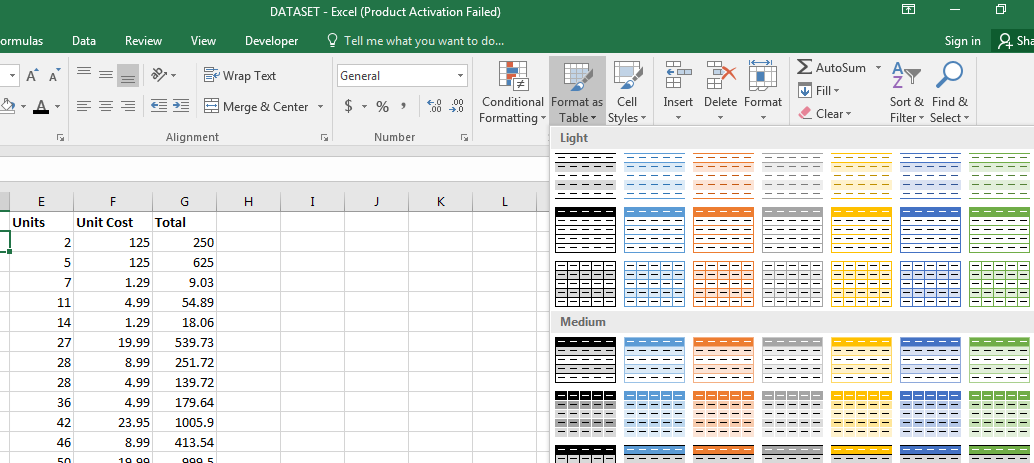
As is often the case in Excel, there is more than one way to do the same thing. I encourage readers to practice using the Design tab in Excel to become more proficient in table formatting. The more you practice, the more comfortable and efficient you will become at utilizing the tools available in Excel to perfect your data presentation. Excel Table Tools is a powerful feature that allows users to easily manage and customize tables within Excel. One important component of the Excel Table Tools is the Design tab, which provides a variety of options for formatting and customizing tables.
The obvious change is that the data was styled, but there's so much power inside this feature. Tables might be the best feature in Excel that you aren't yet using. With just a couple of clicks (or a single keyboard shortcut), you can convert your flat data into a data table with a number of benefits. To add a total row to your table, right click any cell within the table, point to Table, and click Totals Row. To quickly total the data in your table, display the totals row at the end of the table, and then select the required function from the drop-down list. A custom table style is available only in the workbook where it is created.
Automatic table expansion to include new data
When the table is filtered, these totals will automatically calculate on visible rows only. You can toggle the Total Row on and off with the shortcut control + shift + T. First, remove blank rows and make sure all columns have a unique name, then put the cursor anywhere in the data and use the keyboard shortcut Control + T.
Another way to select the table data is to click any cell within a table, and then press CTRL+A. To select the entire table, including the headers and totals row, press CTRL+A twice. For more information, please see How to use Excel table styles. Sometimes, when people enter related data in a worksheet, they refer to that data as a "table", which is technically incorrect. To convert a range of cells into a table, you need to explicitly format it as such.
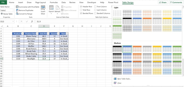
In this tutorial, we will explore the basics of table styles in Excel and how to apply and customize them to enhance the look of your spreadsheets. The best part of this feature is that when you're referencing tables in other formulas, it will automatically include the new rows and columns as well. For example, a PivotTable linked to an Excel data table will update with the new columns and rows when refreshed. A newly created table is already formatted with banded rows, borders, shading, and so on.
If you want to use it in another workbook, the fastest way is to copy the table with the custom style to that workbook. You can delete the copied table later and the custom style will remain in the Table Styles gallery. To apply a new style and remove any existing formatting, right-click on the style, and then click Apply and Clear Formatting. Next, on the Table Design tab, in the Table Styles group, click a table style (hover over a style to see a live preview).
Usually, adding more rows or columns to a worksheet means more formatting and reformatting. When you type anything next to a table, Excel assumes you want to add a new entry to it and expands the table to include that entry. The above script will automatically change the table formatting of all the table objects in the workbook to Table Style Dark 5. If you want to use any other table formatting style, replace the "TableStyleDark5" code element with that specific style code. You can use advanced automation to manage one or different Excel table styles across the workbook.
This includes changing the appearance, adding or removing fields, and arranging the slicers to optimize the user experience. To add a slicer to an Excel table, first select the table or pivot table. Then, go to the "Insert" tab in the Excel ribbon and click on "Slicer." A dialog box will appear, allowing you to select the fields you want to use as slicers. In this section, we will explore how slicers can be used to enhance the functionality of Excel tables and make data analysis easier and more efficient. Filtering data in Excel tables allows you to display only the rows that meet specific criteria, making it easier to analyze and work with the data.
When you convert regular data to an Excel Table, almost every shortcut you know works better. For example, you can select rows with shift + space, and columns with control + space. These shortcuts make selections that run precisely to the edge of the table, even when you can't see the edge of the table. The ability to change table style in Excel is an indispensable data visualization skill.


Comments
Post a Comment